| Oracle® Data Mining Concepts 11g Release 2 (11.2) Part Number E12216-03 |
|
|
View PDF |
| Oracle® Data Mining Concepts 11g Release 2 (11.2) Part Number E12216-03 |
|
|
View PDF |
This chapter describes classification, the supervised mining function for predicting a categorical target.
See Also:
"Supervised Data Mining"This chapter includes the following topics:
Classification is a data mining function that assigns items in a collection to target categories or classes. The goal of classification is to accurately predict the target class for each case in the data. For example, a classification model could be used to identify loan applicants as low, medium, or high credit risks.
A classification task begins with a data set in which the class assignments are known. For example, a classification model that predicts credit risk could be developed based on observed data for many loan applicants over a period of time. In addition to the historical credit rating, the data might track employment history, home ownership or rental, years of residence, number and type of investments, and so on. Credit rating would be the target, the other attributes would be the predictors, and the data for each customer would constitute a case.
Classifications are discrete and do not imply order. Continuous, floating-point values would indicate a numerical, rather than a categorical, target. A predictive model with a numerical target uses a regression algorithm, not a classification algorithm.
The simplest type of classification problem is binary classification. In binary classification, the target attribute has only two possible values: for example, high credit rating or low credit rating. Multiclass targets have more than two values: for example, low, medium, high, or unknown credit rating.
In the model build (training) process, a classification algorithm finds relationships between the values of the predictors and the values of the target. Different classification algorithms use different techniques for finding relationships. These relationships are summarized in a model, which can then be applied to a different data set in which the class assignments are unknown.
Classification models are tested by comparing the predicted values to known target values in a set of test data. The historical data for a classification project is typically divided into two data sets: one for building the model; the other for testing the model. See "Testing a Classification Model".
Scoring a classification model results in class assignments and probabilities for each case. For example, a model that classifies customers as low, medium, or high value would also predict the probability of each classification for each customer.
Classification has many applications in customer segmentation, business modeling, marketing, credit analysis, and biomedical and drug response modeling.
Suppose you want to predict which of your customers are likely to increase spending if given an affinity card. You could build a model using demographic data about customers who have used an affinity card in the past. Since we want to predict either a positive or a negative response (will or will not increase spending), we will build a binary classification model.
This example uses classification model, dt_sh_clas_sample, which is created by one of the Oracle Data Mining sample programs (described in Oracle Data Mining Administrator's Guide). Figure 5-1 shows six columns and ten rows from the case table used to build the model. A target value of 1 has been assigned to customers who increased spending with an affinity card; a value of 0 has been assigned to customers who did not increase spending.
After undergoing testing (see "Testing a Classification Model"), the model can be applied to the data set that you wish to mine.
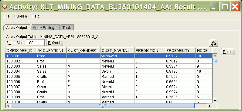
Figure 5-2 shows some of the predictions generated when the model is applied to the customer data set provided with the Oracle Data Mining sample programs. It displays several of the predictors along with the prediction (1=will increase spending; 0=will not increase spending) and the probability of the prediction for each customer.
Figure 5-2 Classification Results in Oracle Data Miner
Note:
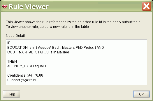
Oracle Data Miner displays the generalized case ID in theDMR$CASE_ID column of the apply output table. A "1" is appended to the column name of each predictor that you choose to include in the output. The predictions (affinity card usage in Figure 5-2) are displayed in the PREDICTION column. The probability of each prediction is displayed in the PROBABILITY column. For decision trees, the node is displayed in the NODE column.Since this classification model uses the Decision Tree algorithm, rules are generated with the predictions and probabilities. With the Oracle Data Miner Rule Viewer, you can see the rule that produced a prediction for a given node in the tree. Figure 5-3 shows the rule for node 5. The rule states that married customers who have a college degree (Associates, Bachelor, Masters, Ph.D., or professional) are likely to increase spending with an affinity card.
Figure 5-3 Decision Tree Rules for Classification
See Also:
Chapter 11 for information about decision trees
Oracle Data Mining Administrator's Guide for information about the Oracle Data Mining sample programs
A classification model is tested by applying it to test data with known target values and comparing the predicted values with the known values.
The test data must be compatible with the data used to build the model and must be prepared in the same way that the build data was prepared. Typically the build data and test data come from the same historical data set. A percentage of the records is used to build the model; the remaining records are used to test the model.
Test metrics are used to assess how accurately the model predicts the known values. If the model performs well and meets the business requirements, it can then be applied to new data to predict the future.
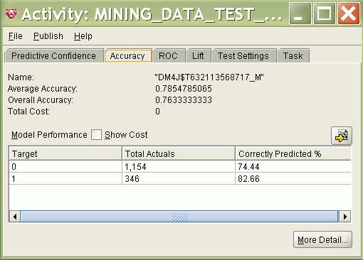
Accuracy refers to the percentage of correct predictions made by the model when compared with the actual classifications in the test data. Figure 5-4 shows the accuracy of a binary classification model in Oracle Data Miner.
Figure 5-4 Accuracy of a Binary Classification Model
A confusion matrix displays the number of correct and incorrect predictions made by the model compared with the actual classifications in the test data. The matrix is n-by-n, where n is the number of classes.
Figure 5-5 shows a confusion matrix for a binary classification model. The rows present the number of actual classifications in the test data. The columns present the number of predicted classifications made by the model.
Figure 5-5 Confusion Matrix for a Binary Classification Model
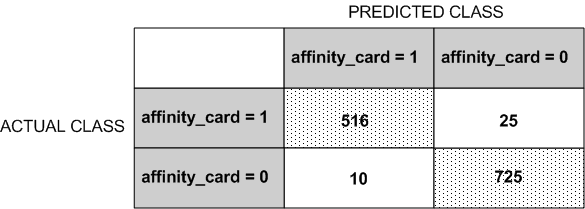
In this example, the model correctly predicted the positive class for affinity_card 516 times and incorrectly predicted it 25 times. The model correctly predicted the negative class for affinity_card 725 times and incorrectly predicted it 10 times. The following can be computed from this confusion matrix:
The model made 1241 correct predictions (516 + 725).
The model made 35 incorrect predictions (25 + 10).
There are 1276 total scored cases (516 + 25 + 10 + 725).
The error rate is 35/1276 = 0.0274.
The overall accuracy rate is 1241/1276 = 0.9725.
Lift measures the degree to which the predictions of a classification model are better than randomly-generated predictions. Lift applies to binary classification only, and it requires the designation of a positive class. (See "Positive and Negative Classes".) If the model itself does not have a binary target, you can compute lift by designating one class as positive and combining all the other classes together as one negative class.
Numerous statistics can be calculated to support the notion of lift. Basically, lift can be understood as a ratio of two percentages: the percentage of correct positive classifications made by the model to the percentage of actual positive classifications in the test data. For example, if 40% of the customers in a marketing survey have responded favorably (the positive classification) to a promotional campaign in the past and the model accurately predicts 75% of them, the lift would be obtained by dividing .75 by .40. The resulting lift would be 1.875.
Lift is computed against quantiles that each contain the same number of cases. The data is divided into quantiles after it is scored. It is ranked by probability of the positive class from highest to lowest, so that the highest concentration of positive predictions is in the top quantiles. A typical number of quantiles is 10.
Lift is commonly used to measure the performance of response models in marketing applications. The purpose of a response model is to identify segments of the population with potentially high concentrations of positive responders to a marketing campaign. Lift reveals how much of the population must be solicited to obtain the highest percentage of potential responders.
The sample lift chart in Figure 5-6 shows that the cumulative lift for the top 30% of responders is 2.22 and that over 67% of all likely responders are found in the top 3 quantiles.
Oracle Data Mining computes the following lift statistics:
Probability threshold for a quantile n is the minimum probability for the positive target to be included in this quantile or any preceding quantiles (quantiles n-1, n-2,..., 1). If a cost matrix is used, a cost threshold is reported instead. The cost threshold is the maximum cost for the positive target to be included in this quantile or any of the preceding quantiles. (See "Costs".)
Cumulative gain is the ratio of the cumulative number of positive targets to the total number of positive targets.
Target density of a quantile is the number of true positive instances in that quantile divided by the total number of instances in the quantile.
Cumulative target density for quantile n is the target density computed over the first n quantiles.
Quantile lift is the ratio of target density for the quantile to the target density over all the test data.
Cumulative percentage of records for a quantile is the percentage of all cases represented by the first n quantiles, starting at the end that is most confidently positive, up to and including the given quantile.
Cumulative number of targets for quantile n is the number of true positive instances in the first n quantiles.
Cumulative number of nontargets is the number of actually negative instances in the first n quantiles.
Cumulative lift for a quantile is the ratio of the cumulative target density to the target density over all the test data.
ROC is another metric for comparing predicted and actual target values in a classification model. ROC, like lift, applies to binary classification and requires the designation of a positive class. (See "Positive and Negative Classes".)
You can use ROC to gain insight into the decision-making ability of the model. How likely is the model to accurately predict the negative or the positive class?
ROC measures the impact of changes in the probability threshold. The probability threshold is the decision point used by the model for classification. The default probability threshold for binary classification is .5. When the probability of a prediction is 50% or more, the model predicts that class. When the probability is less than 50%, the other class is predicted. (In multiclass classification, the predicted class is the one predicted with the highest probability.)
ROC can be plotted as a curve on an X-Y axis. The false positive rate is placed on the X axis. The true positive rate is placed on the Y axis.
The top left corner is the optimal location on an ROC graph, indicating a high true positive rate and a low false positive rate.
Figure 5-7 Receiver Operating Characteristics Curves
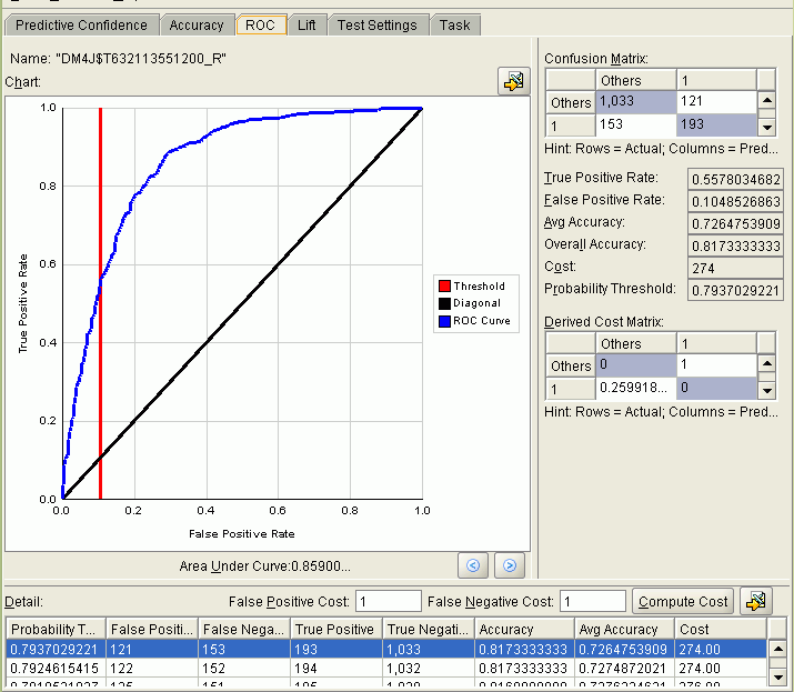
The area under the ROC curve (AUC) measures the discriminating ability of a binary classification model. The larger the AUC, the higher the likelihood that an actual positive case will be assigned a higher probability of being positive than an actual negative case. The AUC measure is especially useful for data sets with unbalanced target distribution (one target class dominates the other).
In the example graph in Figure 5-7, Model A clearly has a higher AUC for the entire data set. However, if a false positive rate of 40% is acceptable, Model B is better suited, since it achieves a better error true positive rate at that false positive rate.
Changes in the probability threshold affect the predictions made by the model. For instance, if the threshold for predicting the positive class is changed from .5 to.6, fewer positive predictions will be made. This will affect the distribution of values in the confusion matrix: the number of true and false positives and true and false negatives will all be different.
The ROC curve for a model represents all the possible combinations of values in its confusion matrix. You can use ROC to find the probability thresholds that yield the highest overall accuracy or the highest per-class accuracy. For example, if it is important to you to accurately predict the positive class, but you don't care about prediction errors for the negative class, you could lower the threshold for the positive class. This would bias the model in favor of the positive class.
A cost matrix is a convenient mechanism for changing the probability thresholds for model scoring.
See Also:
"Costs"Oracle Data Mining computes the following ROC statistics:
Probability threshold: The minimum predicted positive class probability resulting in a positive class prediction. Different threshold values result in different hit rates and different false alarm rates.
True negatives: Negative cases in the test data with predicted probabilities strictly less than the probability threshold (correctly predicted).
True positives: Positive cases in the test data with predicted probabilities greater than or equal to the probability threshold (correctly predicted).
False negatives: Positive cases in the test data with predicted probabilities strictly less than the probability threshold (incorrectly predicted).
False positives: Negative cases in the test data with predicted probabilities greater than or equal to the probability threshold (incorrectly predicted).
True positive fraction: Hit rate. (true positives/(true positives + false negatives))
False positive fraction: False alarm rate. (false positives/(false positives + true negatives))
Costs, prior probabilities, and class weights are methods for biasing classification models.
A cost matrix is a mechanism for influencing the decision making of a model. A cost matrix can cause the model to minimize costly misclassifications. It can also cause the model to maximize beneficial accurate classifications.
For example, if a model classifies a customer with poor credit as low risk, this error is costly. A cost matrix could bias the model to avoid this type of error. The cost matrix might also be used to bias the model in favor of the correct classification of customers who have the worst credit history.
ROC is a useful metric for evaluating how a model behaves with different probability thresholds. You can use ROC to help you find optimal costs for a given classifier given different usage scenarios. You can use this information to create cost matrices to influence the deployment of the model.
Like a confusion matrix, a cost matrix is an n-by-n matrix, where n is the number of classes. Both confusion matrices and cost matrices include each possible combination of actual and predicted results based on a given set of test data.
A confusion matrix is used to measure accuracy, the ratio of correct predictions to the total number of predictions. A cost matrix is used to specify the relative importance of accuracy for different predictions. In most business applications, it is important to consider costs in addition to accuracy when evaluating model quality. (See "Confusion Matrix".)
The positive class is the class that you care the most about. Designation of a positive class is required for computing lift and ROC. (See "Lift" and "Receiver Operating Characteristic (ROC)").
In the confusion matrix in Figure 5-8, the value 1 is designated as the positive class. This means that the creator of the model has determined that it is more important to accurately predict customers who will increase spending with an affinity card (affinity_card=1) than to accurately predict non-responders (affinity_card=0). If you give affinity cards to some customers who are not likely to use them, there is little loss to the company since the cost of the cards is low. However, if you overlook the customers who are likely to respond, you miss the opportunity to increase your revenue.
The true and false positive rates in this confusion matrix are:
In a cost matrix, positive numbers (costs) can be used to influence negative outcomes. Since negative costs are interpreted as benefits, negative numbers (benefits) can be used to influence positive outcomes.
Suppose you have calculated that it costs your business $1500 when you do not give an affinity card to a customer who would increase spending. Using the model with the confusion matrix shown in Figure 5-8, each false negative (misclassification of a responder) would cost $1500. Misclassifying a non-responder is less expensive to your business. You figure that each false positive (misclassification of a non-responder) would only cost $300.
You want to keep these costs in mind when you design a promotion campaign. You estimate that it will cost $10 to include a customer in the promotion. For this reason, you associate a benefit of $10 with each true negative prediction, because you can simply eliminate those customers from your promotion. Each customer that you eliminate represents a savings of $10. In your cost matrix, you would specify this benefit as -10, a negative cost.
Figure 5-9 shows how you would represent these costs and benefits in a cost matrix.
With Oracle Data Mining you can specify costs to influence the scoring of any classification model. Decision Tree models can also use a cost matrix to influence the model build. A build-time cost matrix is specified in the CLAS_COST_TABLE_NAME setting for the model.
With Bayesian models, you can specify prior probabilities to offset differences in distribution between the build data and the real population (scoring data).
Note:
Prior probabilities are specified in a priors table identified by theCLAS_PRIORS_TABLE_NAME setting for the model.
Logistic regression and SVM classification use a weights table, specified in the CLAS_WEIGHTS_TABLE_NAME setting to influence the relative importance of different classes during the model build. See "Logistic Regression".
In many problems, one target value dominates in frequency. For example, the positive responses for a telephone marketing campaign may be 2% or less, and the occurrence of fraud in credit card transactions may be less than 1%. A classification model built on historic data of this type may not observe enough of the rare class to be able to distinguish the characteristics of the two classes; the result could be a model that when applied to new data predicts the frequent class for every case. While such a model may be highly accurate, it may not be very useful. This illustrates that it is not a good idea to rely solely on accuracy when judging the quality of a classification model.
To correct for unrealistic distributions in the training data, you can specify priors for the model build process. Other approaches to compensating for data distribution issues include stratified sampling and anomaly detection. See Chapter 6.
In Oracle Data Miner, the priors option is available when you manually run a classification activity that uses the Naive Bayes algorithm, as shown in Figure 5-10.
Figure 5-10 Setting Prior Probabilities in Oracle Data Miner
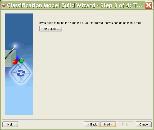
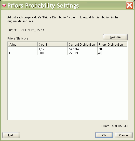
Figure 5-11 shows the Priors Probability Settings dialog in Oracle Data Miner. The prior probabilities have been set to 60% for a target value of 0 and 40% for a target of 1. This means that the ratio of 0 to 1 in the actual population is typically about 1.5 to 1.
Figure 5-11 Priors Probability Settings in Oracle Data Miner
Oracle Data Mining provides the following algorithms for classification:
Decision trees automatically generate rules, which are conditional statements that reveal the logic used to build the tree. See Chapter 11, "Decision Tree".
Naive Bayes uses Bayes' Theorem, a formula that calculates a probability by counting the frequency of values and combinations of values in the historical data. See Chapter 15, "Naive Bayes".
Generalized Linear Models (GLM)
GLM is a popular statistical technique for linear modeling. Oracle Data Mining implements GLM for binary classification and for regression.
GLM provides extensive coefficient statistics and model statistics, as well as row diagnostics. GLM also supports confidence bounds.
Support Vector Machine (SVM) is a powerful, state-of-the-art algorithm based on linear and nonlinear regression. Oracle Data Mining implements SVM for binary and multiclass classification. See Chapter 18, "Support Vector Machines".
The nature of the data determines which classification algorithm will provide the best solution to a given problem. The algorithm can differ with respect to accuracy, time to completion, and transparency. In practice, it sometimes makes sense to develop several models for each algorithm, select the best model for each algorithm, and then choose the best of those for deployment.